
What began as a “silly pastime” of tossing ice chunks down a borehole in Taylor Glacier, Antarctica, has led to a video with more than 8 million views and a collaboration between an acoustics expert and a climate scientist.
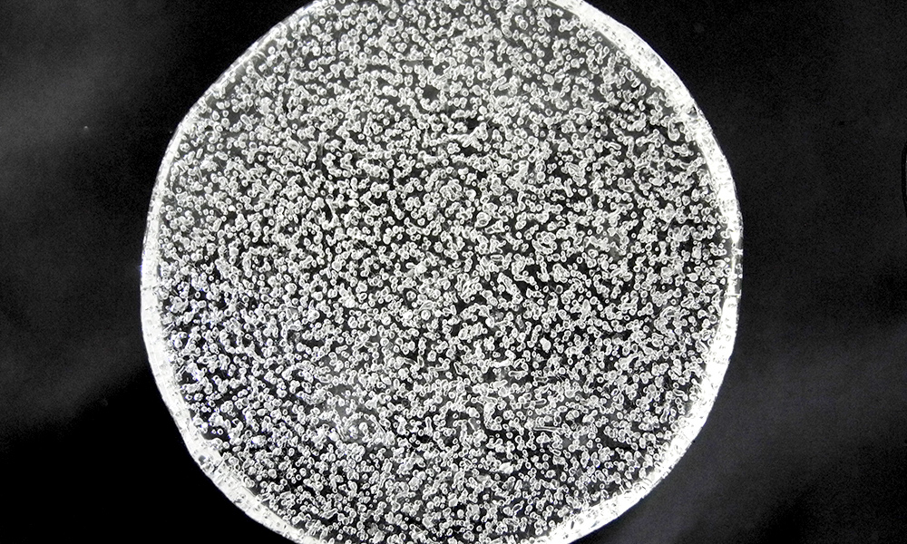
During a research trip to Antarctica, Peter Neff, a postdoctoral associate in the University of Rochester’s Ice Core Lab, recorded a video of the sound ice makes when it is dropped 80-90 meters into a glacier borehole. The video has been viewed millions of times by people across the globe, and Neff received multiple requests from viewers wondering what caused the odd sounds made by the plummeting ice.
??Sound ON??
When #science is done, it’s fun to drop ice down a 90 m deep borehole in an #Antarctic ?? #glacier ❄. So satisfying when it hits the bottom.
Happy hump day. pic.twitter.com/dQtLPWQi7T
— Peter Neff (@peter_neff) February 28, 2018
“In the field we were fascinated by the sound and couldn’t help putting in piece after piece of ice to hear the noises again,” Neff says. “Not being familiar with acoustics, I was only able to wildly guess what caused the sounds.”
Enter Mark Bocko, professor and chair of the electrical and computer engineering department at Rochester. Neff sent him the video and Bocko, too, was intrigued. He quickly got in touch with a number of his Rochester colleagues. Their discussion led to a full analysis of the sound frequencies and, consequently, an in-depth understanding of what causes the noises.
“I had never heard anything like this recording before, especially the ‘ricochet’ sound, and I have to admit that we were stymied for a few days,” Bocko says. “After digging into some of the darker recesses of my old acoustics textbooks, I was able to work out the details and this turned out to be a straightforward but really striking illustration of sound dispersion in acoustic waveguides.”
According to Bocko’s analysis:
- As the piece of ice falls down the hole, it scrapes and bounces off the edge of the borehole. You can hear the frequency of this sound decrease as the ice chunk picks up speed the further down the hole it gets. The decrease in frequency is the Doppler effect, the same effect that causes a car horn to drop in pitch as it drives past you.
- After the ice chunk hits the bottom of the borehole, you can hear a “ricochet” noise, which is caused by the slightly different ways the sound from the impact propagates back up the borehole. The acoustic wave for the “heartbeat” impulses travels straight up the borehole, while the other sound waves bounce back and forth off the side-walls of the borehole on their way up. This causes different frequencies to travel at different speeds. The high frequencies travel fastest and get to the top first while the low frequencies lag behind and arrive later.
- The spacing of the “heartbeat” noises after the ice impacts is determined by the depth of the hole and the speed of sound in air. In this case, the speed of sound in air at -20 degrees Celsius is 318.9 meters/second; it takes sound about half a second to make one round in the 80-meter-deep borehole.
Read Bocko’s full analysis below.
While the noise the ice chunks produce is fascinating, Neff says, he also hopes people recognize that the climate clues the ice provides are just as intriguing. “We go to great lengths to understand how ancient air is trapped in bubbles in glacial ice, providing valuable climate perspectives from the past,” he says. “The science we do in Antarctica is incredibly relevant to our understanding of how the earth system works, but it is also fundamentally beautiful that ancient snowflakes just happen to have been recording how our atmosphere has changed in the past and how we are altering its composition today.”
Analysis of ice borehole acoustic signature
Mark F. Bocko
The unusual sounds made when a chunk of ice is dropped into a deep borehole was recorded in this video made by University of Rochester Earth Scientists working in Antarctica.
There are two interesting features in the sound file that we attempt to explain in this short analysis. The first is the set of downward sweeping pitches that are heard after the ice chunk impacts the bottom of the borehole. The second is the sequence of intense sound impulses heard after the ice-chunk strikes the bottom of the borehole. It is helpful for visualization purposes to display the sound file as a spectrogram, shown in Figure 1. (For those not familiar with a spectrogram, this is a plot of the frequency content of the signal versus time. In the following figure the frequency (from 0 Hz to 5000 Hz) is displayed along the vertical axis and the time is displayed along the horizontal axis, the grayscale indicates the intensity of the sound at each frequency and each instant of time.)
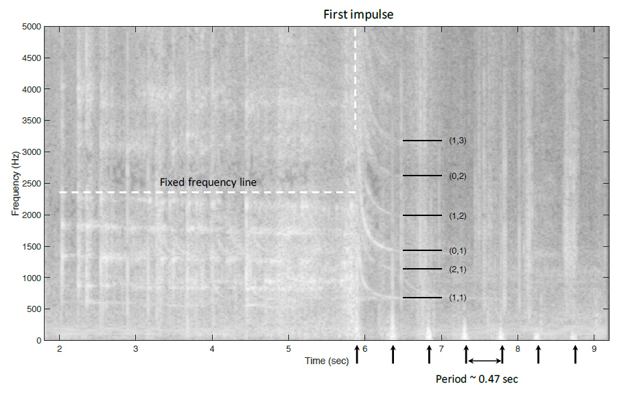
The series of intense impulses following impact are marked with arrows, and the limits of the downward
sweeping pitch tracks seen between 6 and 7 seconds are marked and labeled with corresponding
waveguide mode numbers. A horizontal fixed frequency line is also shown for reference.
We first discuss the sequence of intense low frequency sound impulses marked by the arrows along the bottom of the spectrogram. The arrival of the first impulse at the top of the borehole from impact of the ice chunk hitting bottom is marked by the vertical white dashed line.
Subsequent impulses arrive approximately every 0.47 seconds after the initial impulse – seven impulses are clearly visible in this spectrogram. This observed time delay is the amount of time it takes for the primary sound wave to make one round-trip in the borehole. For a round-trip time of 0.47 sec we estimate the depth of the borehole to be, d = 0.47 *c/2 = 75.3 meters, where we used c = 318.9 m/sec for the speed of sound in air at -20°C. Note that the borehole was reported to be 90 meters deep, but perhaps by the time the video was made enough debris had accumulated in the bottom of the borehole to significantly reduce the depth.
It is more difficult to explain the series of downward sweeping discrete frequency tracks seen in the spectrogram immediately following the first impact (note that at least one such track is seen after the second impact too.) These apparently are due to the excitation of so-called higher-order waveguide modes in the cylindrical borehole. The primary sound propagation mode of a cylindrical acoustic waveguide is one in which the pressure waves have a constant magnitude across a circular cross section of the waveguide. The magnitude of the pressure profile for this mode is labeled (0,0) in Figure 2 below.
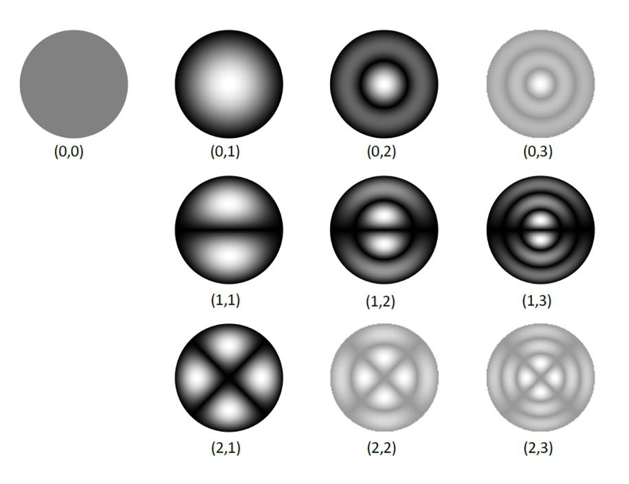
acoustic waveguide with constant circular cross section. The modes evident in the spectrogram are
darkened. The modes not observed in the spectrogram simply were not excited to sufficient energy to be
detectable.
Excitations of the (0,0) mode propagate along the axis of the waveguide at a speed that is independent of frequency, and equal to the speed of sound in free air. The other waveguide modes can propagate only above a cutoff frequency, which is a function of the mode number. The cutoff frequency for each of the waveguide modes can be computed from the diameter, D, of the cylindrical waveguide using the formula,
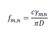
where c is the speed of sound in open air, and ?”$ is the n’th zero of the derivative of the m’th order Bessel function of the first kind – an ugly detail best avoided here. (see Morse and Ingard, pg 513). A table of the cutoff frequencies is given below for a circular waveguide of diameter 10.7 inches (0.2718 m). The diameter was inferred by matching the predicted and observed mode cutoff frequencies from the spectrogram, the inferred value is fairly close to the reported borehole diameter of 10 inches.
Table 1 – The cutoff frequency for selected waveguide modes, assumed waveguide diameter is 10.7 inches.
| Mode (m,n) | Cutoff frequency (Hz) |
| (0,0) | 0 |
| (1,1) | 687.7 |
| (2,1) | 1140.8 |
| (0,1) | 1431.2 |
| (1,2) | 1991.2 |
| (0,2) | 2620.3 |
| (1,3) | 3184.5 |
A plot of the mode group velocity versus frequency is shown for the 6 modes identified in the spectrogram, plus the (0,0) mode which propagates at a constant velocity, the speed of sound in open air.
The speed of propagation of acoustic energy as a function of frequency (the so-called group velocity) for each mode can be represented by a function of the form,
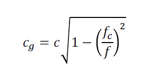
where fc is the cutoff frequency and f is the frequency of the acoustic wave. Note that the group velocity goes to zero below the cutoff frequency, i.e., acoustic energy cannot be propagated by a mode below its cutoff frequency. Far above the cutoff frequency acoustic energy is transported by the mode at the speed of sound in open air, and as the cutoff frequency is approach from above the propagation speed decreases, going to zero at the cutoff frequency, see Figure 3.
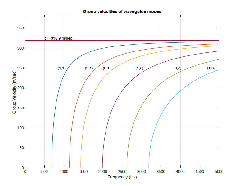
Figure 2.
This is the key to understanding the downward sweeping frequency tracks in the spectrogram. Each track represents acoustic energy being transported by one of the waveguide modes. The high frequency components of the impulsive excitation (when the ice chunk hits the bottom of the borehole) is transmitted at nearly the speed of sound in open air and therefore arrives in coincidence with the main impulse transmitted by the (0,0) mode, which has a constant group velocity equal to c. As the acoustic wave frequency approaches the cutoff frequency for the mode the propagation speed decreases so it takes longer for the acoustic energy to propagate from the bottom of the borehole to the top. That is why the lower frequency components arrive later in time. Note also that below the cutoff frequency of each waveguide mode there is no acoustic energy whatsoever transmitted by the mode, which explains why the frequency track for each mode is asymptotic to the mode cutoff frequency.
It is remarkable how closely the predicted cutoff frequencies agree with the cutoff frequencies observed in the spectrogram. There is only one free parameter in the fit to the data, i.e., the borehole diameter. It is likely that the borehole diameter is slightly greater than the reported 10 inches, and I estimate the bore diameter to be about 10.7 inches, which gives close agreement between the predicted and observed cutoff frequencies.
We note one final interesting feature of the spectrogram, the downward sloping spectral lines that appear from 2 seconds to the time of impact, around 6 sec. On its path down the borehole, the chunk of ice repeatedly hits the walls which excites bending modes of the ice chunk, analogous to the modes of a xylophone bar. Multiple bending modes of the ice chunk are continually excited (and radiating sound) as it falls and bounces off the borehole walls. A horizontal (constant frequency) line is drawn in the spectrogram (see Figure 1) for reference, which makes it easier to see that the frequency of the sound received at the top of the borehole is decreasing as the ice chunk falls down the bore, all the way gaining speed. This is due to theDoppler effect, the same phenomenon that is responsible for the drop in the pitch of a car horn heard by a listener standing alongside the road as a car honking its horn passes by and speeds away.
We refer back to the spectrogram to estimate the shift in pitch for the three most visible tracks over the time interval from 2 sec to 5.8 sec, the frequencies and the inferred speed of the ice chunk at 5.8 seconds is shown in Table 2. To infer the speed of the ice chunk at 5.8 seconds we assume that the speed its speed is near zero initially (@ 2 sec) so there is no Doppler shift initially. The formula to calculate the velocity is then:
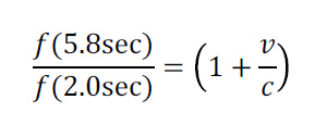 Table 2 – The measured frequencies of bending modes of the ice chunk at 2 sec and 5.8 sec and the inferred velocity at which the ice chunk is falling.
| f(2sec) (Hz) | f(5.8sec) (Hz) | Velocity (m/sec) |
| 2308 | 2102 | 31.25 |
| 1852 | 1690 | 30.57 |
| 1352 | 1235 | 30.21 |
| Average | 30.68 |
If we compute the speed that the ice chunk would attain after falling in the earth’s gravity (g =9.8 m/sec2 for a time interval of t = 3.8 seconds, we find, v = g*t = 37.24 m/sec, which is somewhat larger than the inferred speed from the Doppler shift measurements, but this is not surprising as the ice chunk loses energy and speed each time it bounces off the borehole wall on its way down.
References:
Morse, Philip McCord, and K. Uno Ingard. Theoretical acoustics. Princeton university press,
1968, pp 509 – 514.
Skudrzyk, E. “The Foundations of Acoustics: Basic Mathematics and Basic Acoustics. Wien.”
(1971), pp 430-435.


